Most of my PhD research involved Gaussian Processes. An extremely short summary of Gaussian Processes—written in ML vocab—goes as follows. Consider a training set, $(X_1,Y_1)$ and a test set of inputs, $X_2$. We can write the predicted outputs, $\hat{Y}_2$ as the product of two special matrices and $Y_1$. Specifically
$$ \hat{Y}_2 = \Sigma_{21} \Sigma_{11}^{-1} Y_1 $$
These special matrices are determined by a covariance function, $K$. Exactly how $K$ creates $\Sigma$ will be shown in code and discussed briefly below.
A lot of research in Gaussian Processes involves defining a mathematically valid $K$ with various nice properties. However, we’re going to ignore these considerations in this post and just try to build $K$ (and thus $\Sigma_{21}$ and $\Sigma_{11}$) using a Neural Network and see how it performs on a prediction task.
A Gaussian Process Neural Network Architecture
In general, $K$ is a function that takes in two $X$ points and outputs a number. If $K$ is a covariance function, that number is the covariance between two random variables situated at those two $X$ locations. The $\Sigma$ matrices then are covariance or cross-covariance matrices capturing all pairwise relationships between random variables situated at the $X$ points.
I architect the neural network in the same way. The neural network will take vectors of features and constructs the appropriate $\Sigma$ matrices. I also define $K$ to be a function on point differences. That is, if I have $X_a=(1,1,1)$ and $X_b=(1,−1,0)$, their difference, $(0,-2,-1)$, is input into the next layers of the network. This structure should enable our network to better establish the general phenomenon that points that are close together should have similar Y values.
After taking pointwise differences, $K$ is modeled as a simple densely connected network with a single hidden layer using a tanh activation and a final layer that linearly combines/averages the hidden units. And finally I push everything through an exponential function to achieve the tapering off needed in any covariance function.
The loss function is squared error loss. This is not a standard way to train a Gaussian Process. Most Gaussian Processes are fit by maximizing some version of a multivariate gaussian likelihood. However, I avoid maximizing a likelihood because our $K$ won’t be guaranteed to have the nice aforementioned mathematical properties (positive definiteness), making the Gaussian Likelihood difficult to evaluate. From a pure statistical or mathematical perspective, this is a significant weakness in this approach.
The graph:
## Define inputs
ndim = 3

input_loc = tf.placeholder(tf.float32,[None,ndim])
input_val = tf.placeholder(tf.float32,[None,1])

output_loc = tf.placeholder(tf.float32,[None,ndim])
output_val = tf.placeholder(tf.float32,[None,1])

learning_rate = tf.placeholder(tf.float32,1)

## to better ensure invertibility of Sigma_ii, we add a small
## identity matrix to it, defined by the parameter `nugget_size`
nugget_size = tf.placeholder(tf.float32,[1])

## Develop K
## K takes in two vectors of points, diffs them and applies a wide, dense, one
## hidden layer network to the differences.
## To plug K into our prediction equation, we need to develop both Sigma_ii
## and Sigma_oi, the "covariance" matrix of the input points and the
## cross-covariance matrix between the output and the input points.

## Generate the difference matrix for Sigma_ii
## Some high-dimensional reshape magic needed to produce a correct diff
loc_mat_ii = tf.reshape(input_loc,[1,tf.shape(input_loc)[0],1,ndim])
loc_mat_ii = tf.tile(loc_mat_ii,[tf.shape(input_loc)[0],1,1,1])
t_loc_mat_ii = tf.transpose(loc_mat_ii,[1,0,2,3])
diff_mat_ii = loc_mat_ii - t_loc_mat_ii


## With the difference matrix calculated, we connect it to the hidden layer
## Multiplication broadcasting simplifies this operation significantly
h_dim = 20
h_w = tf.Variable(tf.random_normal([h_dim,1,1,1,ndim],stddev=0.5))
h_b = tf.Variable(tf.random_normal([h_dim,1,1,1],stddev=0.5))

h_ii = tf.nn.tanh(h_b + tf.reduce_sum(h_w * diff_mat_ii,axis=4))

o_w = tf.Variable(tf.random_normal([h_dim,1,1,1],stddev=0.5))
o_b = tf.Variable(tf.random_normal([1],stddev=0.5))

s_ii = tf.reshape(tf.reduce_mean(o_w * h_ii,axis=0) + o_b,
                     [tf.shape(input_loc)[0],tf.shape(input_loc)[0]])

nugget_matrix = tf.diag(tf.tile(nugget_size,[tf.shape(input_loc)[0]]))

s_ii = tf.exp(-s_ii) + nugget_matrix
s_ii_inv = tf.matrix_inverse(s_ii)

######
## generate Sigma_oi using the same parameters to make Sigma_ii

iloc_mat_oi = tf.reshape(input_loc,[1,tf.shape(input_loc)[0],1,ndim])
iloc_mat_oi = tf.tile(iloc_mat_oi,[tf.shape(output_loc)[0],1,1,1])

oloc_mat_oi = tf.reshape(output_loc,[1,tf.shape(output_loc)[0],1,ndim])
oloc_mat_oi = tf.tile(oloc_mat_oi,[tf.shape(input_loc)[0],1,1,1])
oloc_mat_oi = tf.transpose(oloc_mat_oi,[1,0,2,3])


diff_mat_oi = iloc_mat_oi - oloc_mat_oi

h_oi = tf.nn.tanh(h_b + tf.reduce_sum(h_w * diff_mat_oi,axis=4))
s_oi = tf.exp(-tf.reshape(tf.reduce_mean(o_w * h_oi,axis=0) + o_b,
                     [tf.shape(output_loc)[0],tf.shape(input_loc)[0]]))

pred = tf.matmul(s_oi,tf.matmul(s_ii_inv,input_val))
loss = tf.reduce_mean(tf.square(pred - output_val))
I also limit the step size of our Gradient Descent. This added a fairly significant amount of extra TensorFlow code that I don’t include here.
Fitting to data and comparing to other methods
I fit this model to a classical spatial statistics dataset, the Irish Wind dataset by Haslet and Raftery (1989).
The Irish Wind dataset is a remarkably complete dataset of daily wind speeds taken at various monitoring sites in Ireland from 1961-1978. Like other analysts, I pre-processed the data by removing seasonal trend, taking square roots and then centering and scaling the data. Also like other analysts, I remove the Rosslare station from the dataset due to its more erratic data. My ultimate dataset is here.
Before fitting the Neural Network model, I setup a comparison model. A simple covariance model that works decently well with this dataset is an exponential covariance:
$$ K(X_a, X_b) = \phi \exp(-\|D(X_a - X_b)\|) $$
where $\phi$ is a positive number controlling the variance and $D$ is a diagonal matrix essentially scaling distance according to the different dimensions of time and space (for example, a one unit change in space could be extremely different than a one unit change in time). For the immediate comparison, all parameters are 1.
Fit and compare the Neural Network model to the exponential model:
steps = 10000
nreports = 1000

errs = 0
errs_exp = 0

for i in range(steps):

        ## For each update, get a new sample of training and test datasets
        ## n_input and n_output control the number of points in X_1 and X_2
        ## offset controls which day to center our samples around. This is
        ## important because 100 random points distributed in the 70,000
        ## point dataset will on average be very far apart and thus effectively
        ## independent, making training difficult
        n_input = np.random.randint(50)+2
        n_output = np.random.randint(50)+2
        offset = np.random.randint(6000)
        dat_input = gen_wind_data(n_input,offset)
        dat_output = gen_wind_data(n_output,offset)

        ## With the data, run through the graph, update coefficients and record
        ## accuracy.
        _,err = ses.run([sgd_apply,loss],feed_dict={
                input_loc:dat_input['x'],
                input_val:dat_input['y'],
                output_loc:dat_output['x'],
                output_val:dat_output['y'],
                nugget_size:[0.0001],
                learning_rate:[0.1]})

        ## With the same data, calculate squared error using exponential covariance
        err_exp = sq_err_exp_cov(dat_input['x'],
                                 dat_input['y'],
                                 dat_output['x'],
                                 dat_output['y'])

        ### Sum errors and report periodically
        errs_exp = errs_exp + err_exp
        errs = errs + err
        if ((i+1) % nreports) == 0:
            print(errs/nreports, "::", errs_exp/nreports)
            errs = 0
            ert = 0
Outputs:
3.44581754509 :: 0.700560172857
0.573005594732 :: 0.702981137784
0.581162170459 :: 0.703066291396
0.578531336965 :: 0.709449559103
0.559306852582 :: 0.695632392696
0.560115869343 :: 0.697186173774
0.566493079818 :: 0.70041902761
0.556554989581 :: 0.692550035019
0.569026094928 :: 0.706376862357
0.545988285017 :: 0.685677843118
The neural network model outperforms the exponential model, achieving around 20% better squared error performance. This turns out to be no small feat. Optimized $\phi$ and $D$, only gives a 0.5% improvement in squared error. Similarly, there is only a 10% improvement of the exponential model over the squared exponential model (or Gaussian model), where the squared exponential model is usually deemed extremely unnatural.
Visual comparison of ‘covariance’ functions
Given that the ‘covariance’ function given by the neural network performs better than the parametric models, let’s plot both $K$ and see what the major differences are.
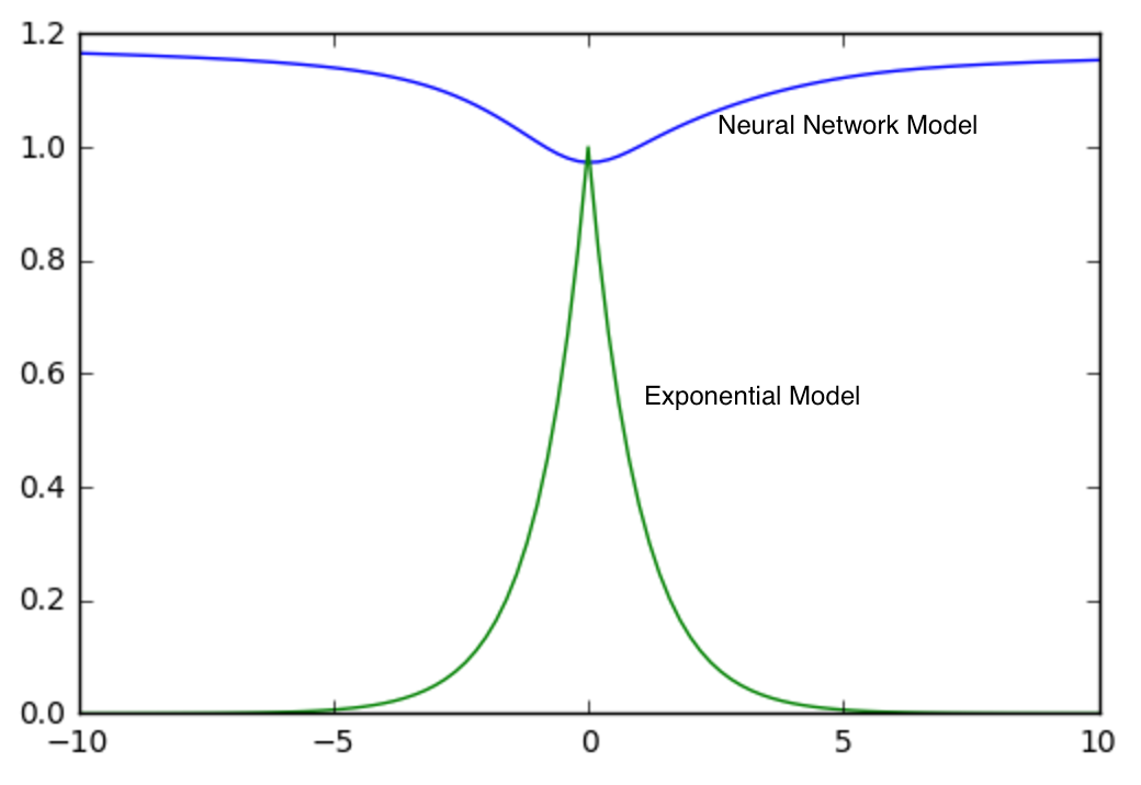
Since all models we considered depend on vector differences, it suffices to generate plots of $K$ in comparison to the origin, $(0,0,0)$. Below is a plot of $K$ for both the neural network and exponential models varying only latitude.
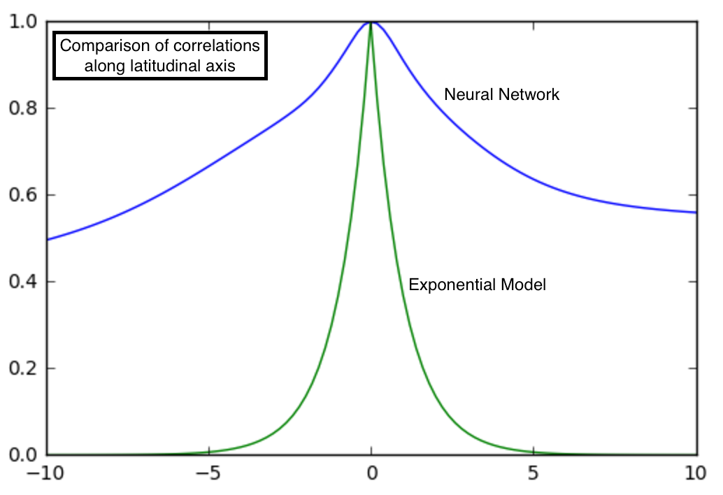
Interestingly, the two models are pretty different. There is much higher ‘correlation’ between points that are a few latitudinal degrees away in the neural network. ‘Correlation’ near the origin is also smoother in the neural network than in the exponential model. For real correlation functions, behavior near the origin is of great interest as it has implications on the smoothness of the process being modeled. However, I caution against reading too much into these differences without a more careful analysis than I provide here.
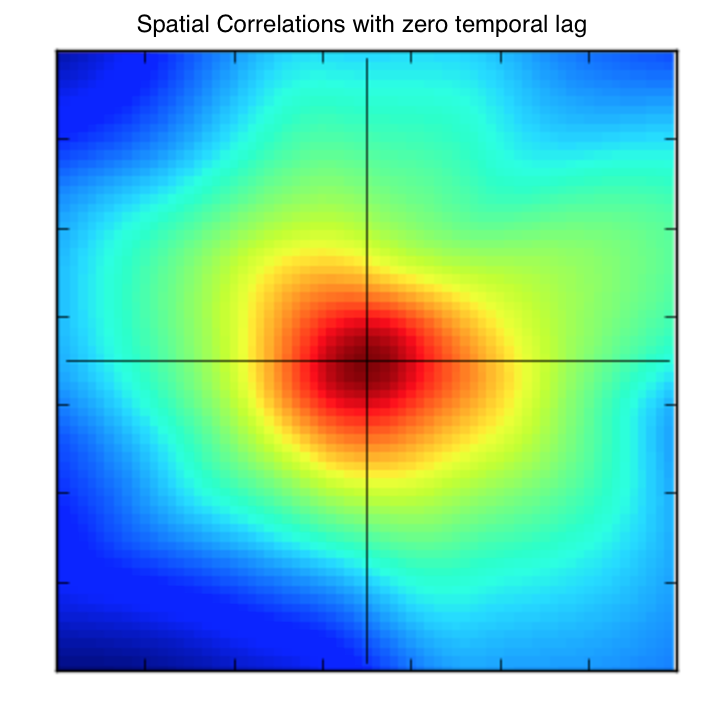
Let’s also consider how these spatial covariances evolve with time. A 2D plot shows the spatial correlations.
Increasing the comparison points by 1 day, we see how these correlations change.
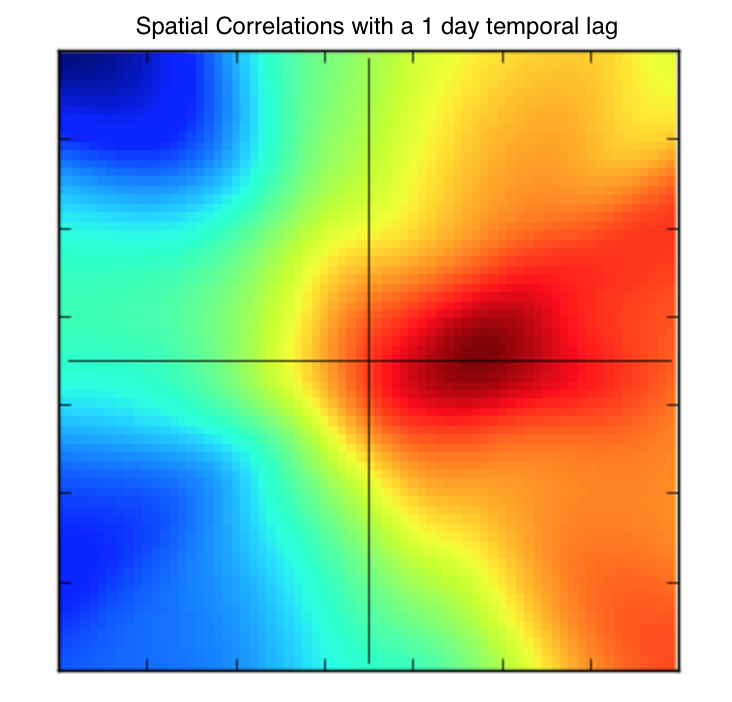
The correlations in time appear the be non-symmetric which can be indicative of a process that drifts. For example, this plot shows that wind speed one day in the future tends to drift eastward and slightly northward. This phenomenon with this dataset has also been confirmed in academic literature as well as intuitively pairs up with the prevailing south-westerly winds of Ireland.
Likelihood comparison
Likelihood comparisons are very common in statistics. Everything else equal, models with higher likelihoods are frequently seen as the better models. The neural network model I made is not positive definite since it isn’t required to be symmetric; however, by symmetrizing the covariance matrix $\Sigma$ by simply adding its transpose and dividing by 2 and also adding just enough on the diagonal to make all eigenvalues positive, a ‘closest’ covariance matrix can be generated with a valid liklihood.
On 10,000 sub-sampled datasets of size 100 the average log-likelihood for the symmetrized neural network model is 46.9 and is 18.0 for the optimized exponential model. This result is perhaps unsurprising given our previous analysis but is still notable that the model generated by the neural network passes this test as well.
You might note that my subsampling method may not be perfect. Ideally I would calculate the likelihood using all datapoints simultaneiously. Unfortunately, this involves working with a massive ~70,000 by ~70,000 matrix, something not possible to work with on standard machinery. A deeper analysis of these models would tackle that problem more directly.
Summary and notes
We built a neural network model that behaves similarly to covariance models. The model had better prediction performance and produced models with higher likelihoods than a common spatial statistics model. The model was also able to accurately identify known structures in the data on its own.
As a final side note, there seemed to be two local minima in the solutions found by the optimization. The most covariance-looking plot was given above. Below is the other solution the network landed on. This function and the more covariance-looking function both had similar performance. But, this function looks exceptionally different than a covariance function. It is unclear to me whether the shape of this function is a trivial transform of the other solution, but it’s worth calling out as a second solution.