When interviewing Data Scientists, candidates will sometimes talk about a recommendation system project and say they used an “SVD” for their model or to fit their model. As a one-time researcher using matrix decompositions heavily, this answer never sat right with me. Strictly speaking, the Singular Value Decomposition (SVD) simply writes an existing matrix in a different way; thus, generating new predictions with an SVD is, on its face, impossible or at least very counter-intuitive.
In attempt to clean up distinctions between Recommendations Algorithms and the classical SVD, I go through both in this post and add an example using a different way to fit a Recommendation model that I found interesting. Since most descriptions of this model use movies as the items being recommended (and following the question in that StackExchange post), I use the terms Movies and Users in this post.
Why the two are conflated
An algorithm related to the SVD was posted by Simon Funk in 2006 as a way to solve the famous Netflix problem. To Simon’s credit, he specifically distinguishes his model/algorithm from the SVD in his post. However, subsequent re-hashings of his approach (for example, this stackoverflow answer) don’t acknowledge the difference.
Details of the Funk model
Let $u$ be a user and $m$ be a movie, and let $r(u,m)$ denote the rating given to $m$ by $u$. The Simon Funk Model asserts that the expected rating $\hat{r}(u,m)$ is equal to the dot product between two vectors plus movie and user biases accounting for say quality of a movie and a general optimisic/pessimistic rating scale of a user. Let $v_u$ and $b_u$ be the vector and bias of a user, and let $w_m$ and $b_m$ be the vector and bias of a movie. Thus:
$$ \hat{r}(u,m) = v_u^Tw_m + b_u + b_m $$
Breaking $\hat{r}$ down in this way is a version of numerical embedding. Essentially, what makes up a user’s preference and a movie’s characteristics are encoded in these numerical vectors and are learned from the data. As a brief example, one dimension in these vectors could represent quality of acting. Users that prize quality acting will have large values for that dimension, and movies with quality acting will also have large values for that dimension. Thus, the dot product combines the user’s preference and the movie’s characteristic to produce an overall higher estimated rating.
The vectors/biases in this model are estimated by considering all known $r(u,m)$ and attempting to minimize squared distance between $r(u,m)$ and $\hat{r}(u,m)$. Funk accomplishes this by initializing all vectors to random values and using stochastic gradient descent with some regularization. This method considers the $r(u,m)$ and $\hat{r}(u,m)$ pairs individually and nudges the corresponding vectors in the right direction to shrink $(\hat{r}(u,m)−r(u,m))^2$.
The SVD analogy to the Funk model
The SVD is a matrix decomposition entirely separate from Funk’s procedure. Details of course are on Wikipeida, but the short version is that the SVD factorizes a known $i\times j$ matrix, $R$, into three parts: $R=USM$. $U$ is an $i\times i$ dense matrix. $M$ is a $j\times j$ dense matrix. And $S$ is a sparse $i\times j$ matrix with only non-zero, non-negative elements in its diagonal.
If we let $S$ be absorbed by either $U$ or $M$ and we trim out all corresponding zero rows or columns, we can write $R=\tilde{U} \tilde{M}$ , where $\tilde{U}$ is an $i\times \min(i,j)$ matrix and $\tilde{M}$ is a $\min(i,j) \times j$ matrix.
Now, let $R$ be the matrix of all user-movie ratings with $i$ users and $j$ movies:
$$ R = \left[ \begin{array}[c c c] ~r(u_1,m_1) & \cdots & r(u_1,m_j) \\ \vdots & \ddots & \vdots \\ r(u_i,m_1) & \cdots & r(u_i,m_j) \end{array} \right] $$
From here, the analogy to Funk’s model becomes more clear. The $a$,$b$-th element of $R$ can be written $\tilde{U}_{a,:} \cdot \tilde{M}_{:,b}$ or as the dot product of two vectors, one corresponding to a row in the $U$ matrix and another corresponding to a column in the $M$ matrix. Thus, we can see that if $R$ is a known matrix, using components of the SVD, we can represent $R$ as the dot product of vectors, much like ratings in the Funk model are the dot product of two vectors.
The comparison between the SVD and Funk’s model gets even more interesting when one considers that chopping last columns off $\tilde{U}$ and last rows off $\tilde{M}$ gives a best (in terms of squared error) low-rank approximation of R. Thus, for example, the best 2 dimensional vector embedding of Users and Movies can be calculated using the SVD by taking only the first two columns of $\tilde{U}$ and the first two rows of $\tilde{M}$.
BUT all this relies on knowing $R$ to start–or in other words already knowing all $r(u,m)$–so, SVD, the matrix factorization, can’t be used for these types of User-Item recommendations directly out-of-the-box.
Fitting the latent user and movie embeddings
So, can the SVD help us directly estimate these useful User and Movie embedding vectors? The short answer is no.
Below I review how to fit these embedding vectors using both Funk’s method and a competing method I came across while analyzing this problem called Alternating Least Squares.
The Funk optimization algorithm (SGD)
If we index the known ratings by $k$ and let the corresponding user and movie indices be $i(k)$ and $j(k)$ respectively, then more or less the specific loss function Funk attempts to minimize is a regularized squared error.
$$ \sum_k (\hat{r}_k - r_k)^2 + \lambda \left(\|v_{u_{i(k)}}\|^2 + \|w_{m_{j(k)}}\|^2 + b^2_{u_{i(k)}} + b^2_{m_{j(k)}} \right) $$
Taking derivatives of this expression with respect to the individual parameters in the v and w vectors gives the equations on Funk’s page.
SGD competitor: Alternating Ridge Regression
If you consider only the user parameters or only the movie parameters, re-arranging data shows that this loss function is exactly linear regression with an L2 regularization–or in other words, Ridge Regression.
Consider a single user, $u$ and all the movies rated by $u$: $m_1,\cdots,m_{j(u)}$. Consider the following matrix, $X$, and vectors, $Y$ and $\beta$:
$$ X:=\left[\begin{array}{cc} 1 & w^T_{m_1} \\ \vdots & \vdots \\ 1 & w^T_{m_{j(u)}} \end{array}\right]~~ Y:=\left[\begin{array}{c} r(u,m_1) - b_{m_1} \\ \vdots \\ r(u,m_{j(u)}) - b_{m_{j(u)}} \end{array}\right] ~~ \beta := \left[\begin{array}{c} b_u \\ v_u \end{array} \right] $$
With this re-arrangement, we can represent all components of our loss function involving $v_u$ or $b_u$ as a ridge regression:
$$ \|X \beta - Y \|^2 + \lambda \| \beta \| ^2. $$
Moreover, Ridge Regression can be solved analytically as
$$ \mbox{argmin}_\beta \|X \beta - Y \|^2 + \lambda \| \beta \| ^2 = \left(X^TX + \lambda I\right)^{-1} X^TY $$
Thus, for given movie vectors, movie biases and $\lambda$, we can calculate optimal user vectors by solving a ridge regression for each user.
Re-arranging the $X$ and $Y$ matrices for movies, we can find that the same statement holds true for movie vectors and biases. We can calculate optimal movie characteristics given user preferences by solving a ridge regression for each movie.
A procedure that repeatedly solves for user preferences, then movie characteristics (or some combination thereof) therefore may minimize our loss more effectively than the SGD method from Funk. Based on our numerical experiments, we find this to be the case. Due to the alternating nature of this procedure, the original discoverers called it Alternating Least Squares (ALS). Since this discussion solely used Ridge Regression, I here refer to it as Alternating Ridge Regression (ARR).
Outperforming SGD with ARR
To show ARR is effective, we apply it to a dataset of User-Movie Recommendations. Specifically we apply it to the MovieLens 100k dataset. This dataset can be downloaded freely at that link or can be downloaded through use of the Surprise package in Python. We will be making comparisons to the Recommendation algorithms in the Surprise package.
Since ARR and SGD are both ways to fit the same model, we compare: training set loss, test set loss and computation time. The SGD implementation we use is that used in the Surprise package. Our ARR approach is implemented in Python.
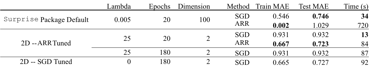
Results show (1) ARR minimizes training loss extremely effectively, though this leads to overfitting and (2) heavy regularization under a ARR can give a performant model even in only 2 dimensions. Indeed the best ARR test loss using 2D vectors outperforms the majority of the best methods in the Surprise package on this dataset as a whole, even though those methods use 100 dimensions and a more complicated model.
Of course, SGD still does well. It remains a robust way to estimate User and Movie embeddings such that the estimated embeddings work well on a hold-out set. In contrast, although ARR can obtain extremely good Training Set performance, it much more easily over-fits. The big difference seen between performance of these minimizing algorithms may come down to the fact that SGD itself is sometimes seen as a method of regularization. Solutions found by SGD usually cannot be overly sharp. In part we saw this in an earlier post.