Almost all Deep Learning models are fit using some variant of Gradient Descent. Adam, RMSProp, basically every optimizer in the below auto-complete relies on some clever averaging or momentumizing gradients or learning rate adaptations.

In this post, I’m going to train a Neural Network not using Gradient Descent. I will be using something closer to Gradient Boosting. I call it Gradient Fitting.

Gradient Boosting review

First, an extremely short description of Gradient Boosting. The standard regression problem tries to calculate

$$ \hat{f} = \mbox{argmin}_{f \in F} L(f(X),Y) $$

for some function class, $F$, and loss function, $L$. Gradient Boosting solves this by looking at $\partial L/ \partial f$–the vector of derivatives of the loss with respect to the predictions–fitting essentially an adjustment $f_i$ so that

$$ \hat{f}_i = \mbox{argmin}_{f \in F} \left\| f(X) - \frac{-\partial L}{\partial f} \right\|^2 $$

Then the solution to the main problem is just the weighted sum of the adjustments:

$$ \hat{f} = \sum_i \alpha_i \hat{f}_i(X) $$

where the weights are determined by conducting a line search to minimize $L$ at each iteration when adding $\alpha_i \hat{f}_i(X)$. Alternatively one can think of the αi as a variable learning rate. In short, Gradient Boosting is a kind of Gradient Descent but in a restricted function space.

Can Gradient Boosting fit weights for my Deep Network?

Yes. A key observation I will make use of is the fact that the most common nodes in a Neural Network take in some kind of $X$ as an input and then outputs an $X\beta$ through an activation function, where $\beta$ are the set of weights being trained in the network.

For example, densely connected nodes and convolutional layers both follow this pattern.

Consider a dense network input to some loss

$$ L(g(f(X\beta)\gamma), Y) $$

where $g$ and $f$ are activations taken elementwise. $X$ here is an input matrix and the weights to be trained are $\beta$ and $\gamma$. If I write $X\beta$ as $Z_1$ and $f(X\beta)\gamma$ as $Z_2$, I can take derivatives of $L$ with respect to these intermediate values and update the weights similar to boosting.

$$ \beta_{adj} = \mbox{argmin}_\beta \| X\beta - \frac{-\partial L}{\partial Z_1} \|^2 $$ and $$ \gamma_{adj} = \mbox{argmin}_\gamma \| f(X\beta) \gamma - \frac{-\partial L}{\partial Z_2} \|^2 $$ then $$ \beta_{new} = \beta_{old} + \alpha \beta_{adj}; ~~~ \gamma_{new} = \gamma_{old} + \alpha \gamma_{adj} $$ where $\alpha$ can be treated like a learning rate or picked using a line search.

With some empirical experiments, the above update is usually improved by using an L2 regularization, making the adjustments solutions to a ridge regression rather than a linear regression.

Why do this?

Per a previous post, Gradient Descent doesn’t work on problems as simple as linear regression. This does.

Also of note, Ali Rahimi talks of similar frustrations in his NIPS 2017 talk. This method matches his referenced method, Levenberg-Marquardt (1944), when a single layer and activation is used. As far as I can tell Gradient Fitting presented here is novel. However, others have applied Levenberg-Marquardt to Neural Networks in a different way.

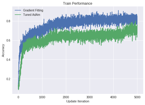
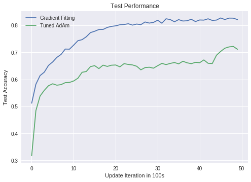
Does it work in practice?

Yes. On a simplified LeNet network, it trained to better optima on both training and test sets.

But does it converge in theory?

Under too-strict-for-deep-learning assumptions, it does. You can view the update as a solution to a majorizing function for a lipschitz convex loss if the input is the entire dataset. Under this view, results in Mairal (2013) prove convergence and give rates.

To extend to the stochastic setting (where batches are used instead of the entire dataset), stochastic theory for quasi-newton methods will apply, but I was unable to find general enough results for this setting in the literature.

Bonus: you can put trees in the first layer of your network

Based on this framework, there’s no reason why the first layer taking the data $X$ as an input can’t be a tree as it is in boosting. Using the above notation, this means instead of fitting $\beta_{adj}$, an $\hat{f}_i$ is fit to $-\partial L/\partial Z_1$, and all the other associated equations stay the same. More on this to come.